An interesting application of silicon photonics is building signal processors, where one can adjust the amplitude and phase of a on incoming signal by utilizing properties of waveguides, combiners, etc. One such example of a signal processing function we might care about is the Hilbert Transform.

But what exactly is the Hilbert transform? Reading the wikipedia page can give a little insight, but is kind of mathy. The basic idea is the Hilbert transform just takes a signal, and simply applies a 90 degree phase shift. How could this ever be useful though, you’re just shifting the phase, doing nothing to the amplitude? This is hardly a useful operation right?

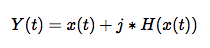
Maybe it is. If we take the Hilbert transform of an arbitrary signal x(t) we get H(x(t)), a phase shifted version of x(t). What if we build a function Y(t) out of these two things? Such a function would look like:

We already said the Hilbert transform is just applying a 90 degree phase shift so this function is really just:

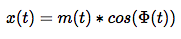
What we have done here is taken a time domain signal x(t) that was purely real and extended it into the complex plane. This is called creating an analytic function. From this analytic function many things are possible. The most common example is carrier recovery in a reciever system. In a communication system we commonly recieve a signal:

If we create an analytic function out of this the result is:

The amplitude m(t) can be recovered as:

One shouldn’t concern themselves with the exact function H(x(t)), there are simple lookup tables, or functions in your favorite programming langauge to easily compute the actual transform (It’s just a simple convolution).

Likewise the instantaneous phase and frequency can also be recovered by the normal arctan/differentiation methods. We can mathematically remove the carrier and identify the message signal, just by applying the Hilbert transform.

Ok great, so what does this have to do with optics?

This post greatly borrows from here.